Wednesday, December 22, 2010

Python as an Alternative to Lisp or Java, Peter Norvig revisited

Because I'm a fan of Peter Norvig, and because I've recently been going through some of his articles about Lisp, I ran into an old entry of his from 1999 about Lisp and Java. In it, he links off to a study where a sample problem was provided in order to compare the efficiency of C++/Java programmers. Feel free to read his post Lisp as an Alternative to Java. How did Peter do 11 years ago?

I did not participate in the study, but after I saw it, I wrote my version in Lisp. It took me about 2 hours (compared to a range of 2 to 8.5 hours for the other Lisp programmers in the study, 3 to 25 for C/C++ and 4 to 63 for Java) and I ended up with 45 non-comment non-blank lines (compared with a range of 51 to 182 for Lisp, and 107 to 614 for the other languages). (That means that some Java programmer was spending 13 lines and 84 minutes to provide the functionality of each line of my Lisp program.)

While relaxing a bit while testing was going on for our code push today, I followed the same instructions, only in Python. I hadn't read his lisp code before (and reading it afterwards, there is a lot of Common-Lisp-isms that I don't really understand), nor had I read the specific problem before (though I solved a similar problem in the spring of 1999 during a local programming competition in undergrad in C++).

My first correct solution was done in an hour with 53 non-comment lines, but I could trim it to 37 lines if I was okay collapsing all lines that could be collapsed.

Looking around a bit while counting lines, I realized that if I added a utility function, I could remove some confusing stuff, while at the same time reducing line count. Spending another 10 minutes got me to 47 lines without comments or spaces, and 44 if I collapsed all lines that could be collapsed while limiting it to 78 columns wide.

My solution is available at this github gist. I didn't write this or this blog post to be "look at how good Python is", because obviously one's ability to program solutions to problems/puzzles/etc., is fundamentally related to your experience and ability to think in a given language. And, on the most part, I've been living and breathing Python for the past 10+ years, with the last 6 years programming 4-5 days a week in Python both professionally and personally. That said, I do think that similar conclusions can be drawn from this bit of the experiment as Peter made, primarily that Python is very effective, very expressive, and can cut out a lot of the bullshit that most Java programmers deal with on a regular basis.

UPDATE:
A commenter pointed out that I had a bug that was exposed running over the large input files and comparing with the large output file. I fell into the same ambiguity as was pointed out in the paper as the "hint" on page 12.

If you want to see more posts like this, you can buy my book, Redis in Action from Manning Publications today!

Friday, October 29, 2010

Being a student isn't easy, it requires actual work

Wandering about the internet this morning prior to doing some actual work, I happened upon a blog post by Seth Goodin about teaching, and how students should demand better instruction. Historically, I've generally agreed with and enjoyed Seth's blog (though lamenting being unable to comment there directly), but in this case, I think he's missing the point.

I can certainly appreciate the plight of college students everywhere, spending tens of thousands of dollars to go to school. I did the same thing for my college years, and even continued for another 5 1/2 years to go to grad school. Almost three years out of it, and I've still got loans, and probably will for a few years to come (9 1/2 years of postsecondary education isn't cheap in the states). However, I had the pleasure of being taught by amazing professors at both institutions that I attended, but even more importantly, attended school with interested and engaged students (I wasn't the only one doing homework on Friday nights). Sadly, this isn't always the case...

Everyone agrees that if you have a poor teacher/professor, your learning (and grades) will suffer... but there's a limit to which that is the instructor's fault. So often when I was both studying and teaching, I would hear complaints (and offered a few myself) about a poor instructor. Either they didn't care, didn't understand where their teaching fell on deaf ears, taught something unrelated to the course, ... However, when confronted with this type of instructor, a student is given an opportunity to engage themselves in learning. Classes come with books, and instructors are meant to help the student understand and integrate the knowledge and wisdom within those books. But prior to the internet, Wikipedia, or Khan Academy, students have managed to learn, despite poor instructors. How? They read and studied the books, consulting their fellow and elder students when they had questions. I know I was different in this regard, as when I found difficulty understanding my teacher during Trigonometry in high school, I read the book, studied, and understood it. When asked by other students how I managed to do well despite a confusing teacher, I pointed at the book. Only a few of them had taken the time to read the book beyond the problems, or when they did, would take the time to understand it.

Back when I was a TA in grad school, I made many mistakes (mostly in my first couple quarters). But by the final quarter of my teaching stint, I was doing 3 back-to-back sections for the same course, an hour each. The students who showed up and let even just a little bit of my enthusiasm rub off on them were engaged (if you are not excited about what you are teaching, students won't care, and students won't come). But what happened was that 5-10% of students never showed up for any of the discussion sections (except for reviews prior to exams). They would sometimes go to class (sometimes watching television or DVDs in the back rows), read their classmate's notes, hand in half-copied, half-bullshit homework, and expect to learn enough in one hour to be sufficient for an Algorithms/Data Structures midterm/final. Sometimes they managed to cram enough, but usually we would be overly generous and give them a D-.


I can appreciate what Seth is trying to say: expect more from your teachers/professors/instructors. But an amazing instructor can only go so far. Students must also be engaged and willing to participate in the process of learning, otherwise they are at least as much to blame for wasting their time and money as a poor instructor.

If you want to see more posts like this, you can buy my book, Redis in Action from Manning Publications today!

Sunday, October 10, 2010

YogaTable as a Database Server

As promised in my last update, YogaTable is no longer an embedded database. Included in the source is a new server component, which listens for requests on a configurable host and port, defaulting to localhost:8765 .

I have included a client for Python, which has everything necessary for basic and advanced YogaTable use. The protocol is basically JSON over HTTP GET/POST, which makes it straightforward for interacting with using just about any language. I am in the process of documenting what is necessary to write new clients, and will be writing a client for Javascript, as well as a more advanced Python client library. Some simple benchmarks with Apache Bench tell me that YogaTable can perform 60 single inserts/second, and around 2500 bulk inserts/second, but that's in mostly ideal conditions.

One of the features that I am most excited about is being able to script the modification of multiple rows in the database with Lisp. I've taken a merged version of Peter Norvig's lis.py and lispy.py, improved the performance, removed some unnecessary features (some of which were unnecessary for database updates), added some other features, and ... Well, let's just see what it looks like. The following is an example from the YogaTable's tests. It shows how you can transactionally update two rows in the database at the same time, and more specifically, how one could implement transferring money from one account to another.

First, let's set up our rows in the database.
d1 = {'value':decimal.Decimal('200.00')}
d2 = {'value':decimal.Decimal('0.00')}
ids = zip(*self.table.insert([d1, d2]))[0]
d1['_id'] = ids[0]
d2['_id'] = ids[1]

Now, let's set up our shared data, and prepare for the output of our test.
shared = {'transfer':decimal.Decimal('45.23')}
d1['value'] -= shared['transfer']
d2['value'] += shared['transfer']

Let's actually perform the conditional update...
out = self.table.update([
    {'_id':ids[0],
     '__ops':'''
        (load types)
        (define zero (decimal `0.00))
        (define balance (getv `doc `value zero))
        (define transfer (getv `shared `transfer zero))
        (if (>= balance transfer)
            (begin
                (setv `doc `value (- balance transfer))
                (setv `shared `transferred #t)))
        '''},
    {'_id':ids[1],
     '__ops':'''
        (load types)
        (define zero (decimal `0.00))
        (define balance (getv `doc `value zero))
        (define transfer (getv `shared `transfer zero))
        (if (getv `shared `transferred #f)
            (setv `doc `value (+ balance transfer)))
        (delv `shared `transferred)
        (delv `shared `transfer)
        '''}], shared=shared)

The Lisp in here may look a little strange, as some of it is nonstandard. The first few lines of the operations for the rows loads the 'types' module, which offers access to the Python decimal.Decimal datatype (among others), pulls some balance information, and determines how much money is supposed to be transfered. The last few lines in the first operation verifies that there is enough money in the account, then deducts the money, and sets the shared variable 'transferred' to True.

The second operation checks to see if 'transferred' is True, and if so, adds the transferred balance to the second row. The two 'delv' lines in the second operation are merely there to remove the known shared variables so that if someone were to accidentally include a third row, then it wouldn't have access to this data.

And that's it. Money transfers in YogaTable. No need for 2-stage commits.


At this point, you are probably wondering where YogaTable is going as a piece of software. When Google first released AppEngine, one of the things that I was most intrigued by was it's Datastore. Some features I'd never seen before (indexes on all of the values in a list, in particular), and I wished that it was available outside of AppEngine. I'd been meaning to write an AppEngine Datastore-like backend for a long time, and some early versions of YogaTable were actually meant to allow for people to take the Google AppEngine SDK and plug my backend into it. It was meant as a way of scaling the SDK beyond trivial applications, and really, to allow for the full set of features and functionality offered by Appengine's Datastore to people who didn't want to run in Google's datacenters. That is not where YogaTable is going.

After having used MongoDB in production, I realized that the current software offerings for databases was missing something. Something that wasn't tied down to schemas like classic relational databases. Something that wasn't limited if you happened to *only* have a 32 bit machine. Something that could offer enough power for building a moderately-used web site (one million hits/day), but was flexible enough to not get in your way while you were developing it.

And thus, YogaTable was born. Aside from the design requirement of never performing table scans, and it's current lack of built-in replication/clustering, YogaTable today offers sufficient features to get almost any idea from concept to a million hits/day. And with the introduction of a Lisp interpreter, YogaTable is able to offer functionality that is otherwise very difficult in other systems (the simple multi-row update shown above requires a tricky 2-stage commit using AppEngine's Datastore).


There is still work to be done on YogaTable. Mostly, I need to document everything. From there, next steps include replication, clients in a few different languages, support for read-only replicas, automatic master/slave failover, clustering... But all in good time. Documentation first, features next.

I hope everyone stays interested, I know that I'm having fun.

Tuesday, September 14, 2010

YogaTable Part 2: An Embedded NoSQL Database

It's been far too long since my previous post about YogaTable, but in the process of writing tests, testing, and cleaning up some of my original code, I had discovered a few bugs with how some searches were being performed. Throw in some weekend work on Binary Space Partitions, and you have a recipe for a delayed post.

This version introduces an "embedded" interface to YogaTable.  Similar to how SQLite operates, you specify where you would like your tables to be stored, and you receive a Database instance: >>> import embedded; db = embedded.Database(path).  That Database instance has implicitly-defined tables, which can be accessed via db.table_name.insert/ update/ delete/ search/ add_index/ drop_index/... .

Why an embedded database?  Well, for starters, it's a good stepping stone from a storage engine to a full database server.  Once we have an embedded database (especially one with a straightforward interface like YogaTable has), a database serving daemon is just a protocol definition away.  And if you implement your embedded database correctly (like thread safety, etc.), then many of the hard parts relating to multiple clients and routing responses are already solved.

In order to handle index building for new indexes on old data, or index deletion for deleted indexes, and to handle threaded users of the embedded database, we chose to push the processing for each table off into it's own process via Python's convenient multiprocessing library.  Commands are forwarded to each of these processors via multiprocessing.Queue instances (one per table), with all responses for all tables coming back via a single queue.  Threads that make requests against a table don't all wait on the same queue, but each waits on it's own standard Queue.  Responses are routed to the appropriate caller via a special routing thread, which also handles cleanup for threads that have exited.  You can see how routing, process startup, etc., happens in embedded.py.

By pushing all processing into secondary processes, we are also able to leverage multiple processors (with multiple tables or databases) and multiple disks (with multiple databases), which should hopefully reduce latency and increase throughput for heavy users.  We do gain some latency with processes thanks to a serialization and deserialization step for each direction, but the convenience of not needing to write a multi-table load-balancer cannot be understated.  Remember, part of this project's purpose is to build on top of and re-use known-good components whenever we can, and letting the OS handle table-level processor and disk scheduling is the right thing to do.  To see how query processing occurs and how we balance queries with index creation and deletion, check out lib/processor.py.


On the other hand, SQLite has well-known limitations with regards to multiple readers and/or writers.  As in: don't do it (without thinking really hard about it).  So we're not.  Each table processor is single threaded (aside from the effectively transparent communication threads), and has a query-driven event loop.  All requests are processed in-order as they come in to the processor.  When idle, the query processor picks up any outstanding index creation or deletion requests.  The next set of changes will include configuration options to allow for the balancing of request processing vs. indexing vs. cleanup.

If you aren't in the mood for yet another another embedded database, don't worry.  YogaTable is embedded-only just until my next post, whose update will include a RESTful interface for easy multi-language clients, runtime status information, and if I'm feeling frisky, a simple console for querying the database.


On a more personal note, I very much enjoyed building the processing and request routing pieces.  I'd wanted to build a request router for a Linda-like Tuple Space that I had implemented in the fall of 2005 (blog discussion:1 2 3), but that project never made it's way into the real world.  One of the reasons why it never made it's way off my hard drive was partly because of the multiprocessing package, which I saw as a better way of handling tasks for which Linda-like systems were designed.

Tuesday, August 31, 2010

Binary Space Partitions and You

One of the reasons that I do not have the next YogaTable post ready is because I've been spending time dealing with problems relating to geometry.  More specifically, I've had the need to break up some polygons of up to a million points into tiles along a unit grid.

Because of it's convenience, we've licensed GPC and are using it via the Polygon library in Python (GPC is free for non-commercial use, but since this is for work, we had to license it; Polygon is LGPL).  In particular, the Python library has a very simple method for generating tiles of the form we need: Polygon.Util.tile().  Sadly, it is not terribly efficient.  What do I mean?

Say that you wanted to pull one tile from a larger polygon region, using the Polygon library, you would just intersect your desired region with the larger polygon.  That's exactly what you want, and for GPC, is about as optimal as you can get (there are other libraries that offer computationally more efficient polygon intersections, but I've not found any that are as easy to use as GPC).  But what if you wanted tiles?  The algorithm used by Polygon.Util.tile() generates all of the tiles that you want, and performs intersections for each and every one of them.  I know what you are thinking: if the individual operation is optimal, why wouldn't applying the same operation over the larger space be optimal?  Repeated work.

Say we wanted to pull tiles 6a, 6b, and 6c out of the polygon below:
If we were to perform the intersections directly, then we have to trim to the right of column 5 three times, to the left of column 7 three times, and 6 partitions of column 6.  But what if we first performed a simple "trim to the right of column 5" followed by "trim to the left of column 7"?  Well, we would add 4 vertices to the polygon (which we would have needed to add anyways), but by trimming to the left first, we remove 8 vertexes that we never operate on again, as well as another vertex to the right. Over the sequence of operations, we reduce the number of vertexes we need to compute on, and aren't re-performing the same line intersections over and over.

In this simple example, we don't really gain much by partitioning our space, because the shape is so simple.  But by using a very simple algorithm that counts the number of points in each row and column to determine a good row/column to cut the space, we've seen huge returns in our programming investment.  In our case, relatively small polygons of 20-50k points have had their processing time drop from 30-45 seconds to 2-3 seconds.  Our moderately sized polygons of 150-300k points have gone from 15-25 minutes of computation time down to 15-25 seconds.  The killer polygon for us had just over a million points.  It had been running for over 6 hours before I rewrote the algorithm using a simple grid-based BSP algorithm.  We killed the process, and re-ran everything using the updated BSP version.  The entire process completed in under 30 minutes.

I have emailed the author of the Polygon library, so hopefully everyone will have a faster tile for free.  Those of you who can't wait, feel free to get the code from the gist here: http://gist.github.com/560298


ETA: added a link to the Binary Space Partitioning page at wikipedia.

Wednesday, August 18, 2010

Introducing YogaTable, the flexible NoSQL database

In my last post, I talked about building a new NoSQL database from scratch, and how I would describe the decisions I made during it's construction, as well as post code along the way.  This is the first of the series introducing YogaTable.  Strangely enough, the toughest part of all of it was coming up with a name.  At the current revision, insertion, updating, and deletion are all supported, and there are tests.  Querying is not yet in the repository, though I have written the query builder and tests.  Those subjects will be in the next post.


The first design decision I have made with this system is that I will not be building a durable data store; that is, one that offers write-or-fail semantics given modern hardware, handling of system crashes, etc.  It's a hard problem.  Systems which make use of more lazy approaches to durability (like mmap in the case of MongoDB) *will* fail at some point due to the laziness, even ignoring bad disks.  Fixing this issue with replication is great, but it requires more hardware, and in the case of sane underlying systems (real hardware, and/or good virtualization solutions like vmware, xen, etc.), doing it right the first time allows us to not have to band-aid over it with replication.  I will instead use an existing system that does it's absolute best to be durable and transactional by design.

I have also decided that I will not be building a B-Tree indexing system from scratch.  Like the durable data store issue just mentioned, B-Trees are terribly difficult to get right.  So to reduce the amount of time it will take to go from no code to fully-working system, I'm just not going to write a new one.  I will instead use a system that already includes support for B-Tree indexes.

Those of you who know me will already guess that YogaTable will be written in Python, primarily because I know Python better than I know any other language, and secondarily because Python includes all of the tools necessary to build YogaTable out of the box on a modern machine.  In fact, Python includes two transactional data stores with B-Tree indexes as part of the standard library: bsddb.btree and sqlite3.

Because I am not without a sense of irony, and because I have had bsddb.btree bite me with data corruption in the past (when not using the transactional semantics that are not documented in the standard library), I'm going to use Python's interface to SQLite 3, which has been included with the core Python distribution since 2.5 .  As such, YogaTable will be "NoSQL" for the external interface to the database, rather than the actual underlying data store.  Also, because of this choice, it will be fairly straightforward for someone to replace SQLite with another SQL database to offer functionality that I might not have gotten around to adding quite yet (like read-only slaves via MySQL, etc).  Once YogaTable is feature complete (according to my earlier requirements and desires), it is my intent to use this in a small-medium scale production environment for my own projects, fixing bugs as they crop up (or as others report them).

I'm sure someone is going to think and/or point out how backwards it is to use a SQL database to store data for a NoSQL database.  And that's reasonable.  But this world is filled with unsolved difficult programming problems.  I could spend literally months rewriting either the durable data store or the B-Tree index.  On the other hand, I have the utmost respect for those who have already built said systems, and have happily used them in dozens of projects.  Two secrets to software and systems engineering: pick your battles, and stand on the shoulders of giants.  I'm going to do both, at the price of a little SQL.


Now that we have a place to store data and indexes, we've got to decide how it's going to be laid out.  For the sake of simplicity with regards to backup, etc., and because I know a little something about how SQLite 3 works, I'm going to lean towards simplicity.  Each table, information about it's indexes, and the indexes themselves will be stored in a single sqlite3 database file.  This file will have three tables; the data table, the index metadata table, and a single table that includes the index data.  Each table will have various B-Tree indexes over them to ensure that our access patterns are fast.  The general 3-table layout and the db abstraction guts are available in lib/om.py.  Also, as a "new to me" bug, I learned that Python's sqlite3 library doesn't handle list/tuple arguments for 'IN' queries, requiring some str(tuple(data)) shenanigans.

For the index table, we will be prefixing the index data with an index id, which will ensure that we are searching the proper subset of index rows when we search.  Now, we could have placed each index in a separate file, then use SQLite's 'ATTACH DATABASE' command, but then we would have had to query all index tables/databases whenever we perform an update/delete, and that's a pain in the ass (never mind a performance killer whenever we have more than one or two indexes).  We do miss being able to determine the size of each index individually, but that wasn't one of our requirements (though we could keep track of this manually).  For details about how we generate index rows, check out lib/pack.py.

To offer greater flexibility, etc., we will not be storing any Python-centric data in our database.  Data will be stored as JSON, and will be automatically converted to/from JSON by sqlite3 adapters/converters.  Also, for the sake of everyone's sanity, we've included support for dates, datetimes, times, and decimals.  Documentation is forthcoming for future non-Python users to easily convert to/from these formats.  For the impatient, check out lib/adapt.py.


Stay tuned for the next post where I will be discussing the sql query generator, and automatic background index construction.

ETA: updated links to reflect some moved files.

Monday, August 9, 2010

Building a New NoSQL Database from Scratch

Over the course of the last few months, I've been writing a new NoSQL database.  Most readers will laugh and say one of a few different things.  Maybe something like, "NoSQL is a fad", "there are already so many NoSQL options, creating a new one is pointless", or even "unless you bring something new to the table, your adventure is going nowhere".  To sum up my response: yes, it is offering something new.

Every existing SQL/NoSQL solution has tradeoffs.  From the MyISAM storage backend for MySQL (no ACID compliance), to Postgres 8.4 and prior's lack of replication tools (I know I am looking forward to Postgres 9), to secondary index setup/creation in Cassandra, to MongoDB's use of memory-mapped files without transaction log, ... each database trades different advantages for other disadvantages.  For the existing nontrivial noSQL solutions that I have examined (Cassandra, MongoDB, CouchDB, S3, Voldemort, SimpleDB, etc.), I have found that many of my required features are just not available.  In the rare case where my required features were available (Google's AppEngine datastore), it's not available where I need it (Amazon AWS, Slicehost, etc.).

What do I require?

  • scales reasonably on small systems (MongoDB fails here)
  • document/row store (S3 and Voldemort fail here)
  • secondary indexes (SimpleDB fails here)
  • the ability to add/remove indexes during runtime (Cassandra fails here)
  • no surprise queries (aka no table scans, MongoDB, Cassandra, and CouchDB fail here)
  • no corruption on system restart (AWS and other cloud hosting providers sometimes lose your instance for a bit, MongoDB fails here)

Additional points for:

  • no schema (MongoDB, CouchDB, SimpleDB, ...)
  • multiple values per column (MongoDB and AppEngine's list columns)
  • sub-documents (like MongoDB's {'sub-doc':{'attr1':'val1', ...},} )
  • the ability to perform queries against a secondary index while it is being built
  • 10k+ rows inserted/second on modest hardware (MongoDB, ...)
  • replication / sharding / clustering (MongoDB Replica Sets would be optimal)

Astute observers will note that MongoDB offers all of these things, except for scaling well on small systems, and 'no surprise queries'.  To clarify what I mean by both of these; when you are using a 32 bit platform (small Amazon AWS hosts, some smaller VPS machines on other hosts), you are limited to 2 gigs of data and indexes with MongoDB.  This is because they use memory-mapped files as an interface to on-disk files, which limits you to the architecture address space.  As such, MongoDB really only makes sense for relatively small systems, or when you have a 64 bit system.  Further, if you forget to explain your queries in advance (like during ad-hoc queries), to ensure that you are using an index, you can end up scanning your multi-gig database for a simple count query.  On other databases (PostgreSQL and MySQL in the SQL world being the two I am most familiar with), a table scan will slow down other queries, but it won't destroy overall performance.  With MongoDB, that table scan will destroy write throughput for any other operation.  I have run into this myself.

To solve the table scan issue, we need to require an index for every query we perform (this is what Google's AppEngine datastore does).  This somewhat limits ad-hoc queries, but with the ability to add/remove secondary indexes during runtime, and with the ability to make queries against indexes while they are being built (and drop the index during it's creation), we can start an index creation, and immediately perform our query.  If there isn't enough data, we can wait and perform the query again.  Yes, the index building operation does perform a table scan to create the index, but it can be designed to balance itself with incoming queries so that performance doesn't suffer greatly.


Over the course of the coming weeks, I will be documenting the process of building this new NoSQL database from the ground up.  Yes, I said weeks.  Part of the design and implementation will include the use of a readily-available, fast, durable data store (which bypasses many of the nasty implementation details), wrapped with an interface to offer all of the requirements and the first five pluses I list above.  I do have a design for replication/sharding/clustering, but it's the only part of the system I've not built yet.  We'll see how it goes.  I will be posting source on Github as I discuss the design of the system, offering code as the nitty-gritty details of the higher-level design I will describe.

Monday, August 2, 2010

Databases on SSDs, Initial Ideas on Tuning


In the pair of papers on the RethinkDB web site [1] [2], RethinkDB has made a straightforward description of what they have built as a MySQL storage backend, and has alluded to a paper regarding append-only indexes which hasn't yet been posted.  I'm not going to guess at what the paper includes, but I will describe what an applied theorist (like myself) would implement if given the descriptions that they provide.  Note: I am unaffiliated with RethinkDB.

Overall, they have designed a database storage backend around a few primary principles regarding the performance and durability of commercially-available SSDs. 1) Re-writing an existing block of data is slow, 2) writing to an unused block is fast, 3) reading randomly is pretty fast, 4) SSDs have limited lifetimes (so writing/rewriting should be avoided as much as is reasonable), 5) the data storage system should be effectively impervious to failure, 6) recovery from failure should be essentially instantaneous, and 7) backup should be simple.  They go further into the details of their testing on their blog [7], and especially into IO performance based on block size [8] and alignment [9].

Given these principles (some driving their choice, some derived from their choices), they seem to have chosen to use a persistent B-Tree to store their indexes, likely descended from the Sarnak/Tarjan paper regarding persistent search trees [3].  In particular, when writing a row to disk, they also write the B-Tree nodes that would have been modified for the indexes as well (the primary key -> row index, plus whatever other indexes are available), thus offering a "copy on write" semantic for the indexes.  This is what allows for full query-able history of the database at any point in time, and works-around numbers 1 and 4, while offering 5-7, exploiting 2 and 3.  The cost is that as new data and index blocks are written, a fairly large portion of previously-written data becomes historical (compared to more traditional db storage systems), and for most situations, effectively useless.  This wastes space, doesn't allow for the OS to offer "TRIM" commands to the disk to free that historical data, and other annoying things.

One other issue that RethinkDB will likely run into when it starts filling disks (or contending with disks being used for more than just the DB) is write amplification; as blocks are re-used, they must be erased, and on nearly-full SSDs, a simple 4k (or 1 byte) write can result in 128-512k of data writes on the device (depending on the SSD).

To understand what is going on, and why RethinkDB uses 2 gigs to store the equivalent of 50 megs of data and indexes, we first need to look at a toy setup.  Let us imagine that we have 1 million rows of data, each row consisting of two 64 bit integers; a primary key and a secondary data column.  Further, there are two indexes constructed over this data; the primary key index, and an index on the data column.  Given 4k block sizes, back-of-the-envelope calculations would put this at 1 million * 16 bytes for data, and an additional ~1 million * 16 bytes for each of the indexes* (ignoring some metadata and index block headers).

* Leaf nodes of the indexes are the dominant factor here, requiring the value to be indexed, as well as a pointer to the data, for 16 bytes (for a degree 256 B+Tree).  Ancestors which point to leaf nodes account for a little over 1/2 of a bit for every leaf node in a full B+Tree.  To keep our calculations simple, we assume as full a B+Tree as is possible on 1 million nodes.

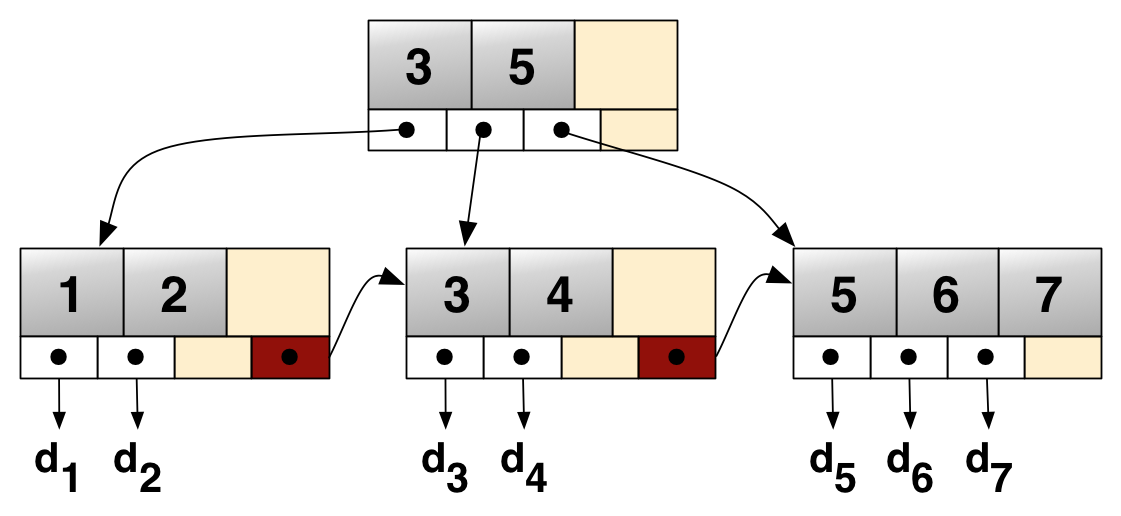
We now have a database that is 48 megs, consisting of data and indexes.  Let's update every key in the database by adding a random integer value to the data column.  For each update, we need to write the new row, update the primary key index to point to the new data row, and update the data index.  In order to update each index, we must copy and update all ancestors of the leaf node in the B+Tree node we update.  To understand why, see the image below.


Ignoring sibling pointers (the d1/d2 block pointing to the d3/d4 block *), in order to write a new d3/d4 block to point to a new d3, we must write a new root block to point to the new d3/d4 block.  For a full tree of 1 million data pointers, the tree is 3 nodes deep, so we must write 3 new nodes for each B+tree index.  We'll give this tree the benefit of the doubt, and say that our increments of the data index are small enough so that, for example, d3/d4 swap places, instead of having d3 migrate to the d1/d2 block.  This still results in 6 block updates for every updated row, even if we assume we can find a place for the new data row of 16 bytes somewhere.

* We can alter the B+Tree format to not have sibling pointers, knowing that any traversal of the index itself will necessarily keep context about the path used to arrive at any block.

After 1 million updates, we will have updated 6 million 4-kilobyte blocks, for a total of 24 gigs of data written to update the index and data.  In a standard database, while more or less the same volume of data would have been written to disk, it would have over-written existing blocks on disk (modulo a transaction or intent log), and would still only use around 48 megs of data.


Reducing Data Writes, Part 1

Because of the read-only nature of the persistent search trees, effectively all updates to the database are transient; data and indexes will be later replaced with some other write.  To reduce wasted space, we should minimize the total amount of data written, which will also minimize the amount of wasted space later.  First, let's reduce the amount of data we write to the index itself, by reducing the size of a logical index block from 4k.  This will result in a deeper tree, but because we can store multiple tree nodes in a single 4k disk block, we can end up updating fewer disk blocks per index update.  

To get an idea of how far this can go, instead of using B+Trees, let's start with a standard binary tree: 64 bit key, 64 bit data pointer (we'll leave our data pointers internal to the tree), 64 bit left/right pointers, for 32 bytes per tree node.  A balanced tree with 1 million nodes is 20 levels deep, which is 640 bytes of index that needs to be updated for every row update for each index.  Heck, we could fit 6x index updates in a single 4k block if we used a binary tree... at the cost of requiring potentially 20 IOs per index lookup to determine our row pointer (10 with caching, based on random tree traversals), vs. 3 for a B+Tree (or 1-2 with caching).

Let's find a balance between a 4k block and a 32 byte block; 512 bytes.  If we squeeze our index into a single 64 bit value, combined with a 64 bit pointer, a B+tree index with 512 byte blocks would be 4 levels deep for our 1 million rows.  Those 4 index blocks of 512 bytes would be 2k, with the data index taking up the second 2k.  Assuming we could find a place for the 16 bytes of data somewhere, those 1 million row updates now only use 4 gigs of storage instead of 24 gigs, and will generally result in 2 IOs when using 16k of cache for each index.


Reducing Data Writes, Part 2

On the one hand, not having or using a transaction log is very useful, it reduces IO, and makes recovery trivially easy: your database is your transaction log.  But let's bring it back, and let's do something crazy: let's either put it on a spinnning disk so we don't worry about writing 16 bytes + metadata to the end of a file whenever we want, or let's put it on an inexpensive flash drive that we write and clear in cycles (alternating between a few of them, to allow for replacement over time), and only ever write full blocks. Let's also include arbitrary "checkpoint" regions (which I'll describe more later).  We'll assume that we're using ZFS with RAIDZ, a RAID 5 array, or some other storage setup where we can rely on the data not being corrupted, while still offering high write throughput.  This is our append-only log.

Whenever we have a row update/insert/delete, instead of modifying the main SSD database, let's instead merely append the modification we want to perform (row with primary key X becomes Y, insert row Y with primary key X, delete row with primary key X, etc.), along with a pointer to the most recent checkpoint, to our append-only log.  Our database engine will keep a cache of all of the rows that have been changed, and for any index rows that we would have updated (as is necessary during writes), we'll instead update them in-memory, without flushing them to disk.

After a fixed number of inserts/updates/deletes, or after a fixed amount of data has been written to the disk (say 1000 rows or 1 meg of data, whichever comes first, which should be tuned on a per-system basis), we dump our row updates and our updated indexes to the SSD with a checkpoint block, and append a new checkpoint to the append-only log.

Whenever the system starts up (on failure, or otherwise), it finds the most recent checkpoint in the append-only log, reads all valid operations after that checkpoint, and replays them as if they were just happening.  By tuning the number of rows/maximum amount of data, we can tune the level of pain we are willing to suffer at system startup.  With the provided 1000 rows or 1 meg of data, even with 512 byte blocks, that is 8000 index read IOs on the SSD to re-play the worst-case log size, which is under 2 seconds on a modern SSD.  Reading 1 meg of data from our append-only log on a spinning disk whould be on the order of 10-30 ms, depending on the latency of our initial seek (assuming a non-fragmented file).

What is to be gained with this append-only log?  After 1000 updates, we reduce the number of root node copy/writes from 1000 to 1.  With 512 byte blocks, we also reduce second level block updates from 1000 to 32.  Third and fourth level block updates may also be reduced, but we won't count those.  That takes us from 1000 4k writes down to 533 4k writes, or really 4megs down to ~2.3 megs.  What if we had stuck with 4k index blocks?  Root node copy/writes go from 1000 to 1, second-level updates go from 1000 to 256.  Overall, from 6000 4k writes to 2514 4k writes, or 24 megs to 10 megs.  Remember, this is for 1000 writes, we'll scale them back up in a minute.

There is a larger proportional difference for the 4k blocks because there are only 3 levels of index, the first of which gets writes reduced by a factor of 1000x, the second which gets reduced by a factor of 4, the third we don't count.  For 512 byte blocks, we get the same 1000x reduction in the root, a better 32x reduction in the second level, but no reduction in the 3rd and 4th levels.

Over the course of those 1 million rows, using this second method on 512 byte blocks, we go from the non-append log 4k block writes of 24 gigs, down to 2.3 gigs, for a factor of better than 10x reduction in data writes to our SSD.

This example was chosen specifically to maximize the ratio of index to data to show effectively worst-case performance on a toy example.  As your data columns grow relative to your index columns, index updates are reduced for insert/update/delete operations.  Generally speaking, we are able to get a 10x or better reduction in data write overhead by combining smaller block sizes with an append-only log file for this toy example.  Real-world use-cases will have different improvements.


Reclaiming Wasted Space

During the course of writing data to the SSD for inserts/updates/deletes, index blocks will become unused (as they are no longer being referenced by the newest index nodes).  Assuming that we are using both earlier described optimizations, whenever we write a checkpoint to the append-only log file, we can include the current number of wasted index blocks.  When applying the updates to create a new checkpoint, any time we are replacing an existing index block, we increment the wasted index block count, and after performing all of our updates, write the wasted index block count as part of the checkpoint.

Remembering our update of the d3/d4 block from before, when we replace the d3/d4 block, we increment the count by 1, and because we need to update the root as well, we increment the count by 1 again.  Generally, this will be the depth of the B+Tree, except in merging nodes and some cases of splitting nodes.

Now that we know how much wasted space we have, and we also know the size of our database file (this is trivially monitored during runtime and during startup).  Whenever we get to a point where we have too much wasted space, we can reclaim that wasted space as follows. 

1. Disable checkpointing in the main process.  This prevents us from having to re-apply the same set of operations on two SSD database files (thus reducing our wasted space and writes to the SSD).
2. In a second process, first copy all of the standard database metadata, then for each table, traverse our primary key index for that table, and write to the a new database file, alternating writing data and index blocks (write all the data for a leaf node in the index, then write that index leaf node, etc.).  In the case of 512 byte blocks, we batch up 8 (or more) data or index blocks to fill our disk block.
3. Continue in the second process to copy all other B+Tree indexes.
4. Signal to the main process that the copy has completed.
5. In the main process, when there are spare cycles, re-apply all of the changes in the append-only log file to the new db in-memory (as per Part 2 above).  Optionally pre-cache hot rows what is in the old database cache.
6. When all of the updates have been performed for the new database file (in memory), perform an atomic filesystem move (discarding the old database file), discard the old database's index cache (from Part 2 above), and discard all other cache.
7. Re-enable checkpointing.

At the point of step #7, the new database file will have everything the old database file had, serving as an online VACUUM.  During this VACUUM operation, system failure is not catastrophic.  At any time before step 5, we can discard the secondary db file.  At any time on or after step 5, restarting the database can use the new database file instead of the old, thus minimizing wasted work.

If we have a database system with relatively low amounts of memory, large amounts of writes, and the memory used by the index cache (from Part 2 above) grows too large, the first process can internally apply a checkpoint to the SSD database (which may fragment the new database file), but not update the append-only file with checkpoint information.  The copying process can then ignore any data written to the main DB file after it has started with it's VACUUM, and the main process just needs to work a little harder in step 5.


In Closing, and Other Notes

I hope that you have a better understanding about the kinds of enhancements that could be done to improve a database storage system to make something like RethinkDB work as well as it does.  I'm guessing that they are using at least one or two ideas described in this post, and I hope that this post gets other people thinking about ways to make such a system even better.  After having seen the performance numbers for a tuned SSD system (flash, drive controller, drive-level caching, kernel drivers, os-level caching, and application), it makes the current 10k Iops numbers for consumer-level devices look like a kids toy.  That RethinkDB is looking for people with heavy DB and kernel experience makes me believe that they will have a great product soon.

Incidentally, after outlining the content of this post, and between writing Part 2 and Reclaiming Wasted Space, I noticed that SQLite 3.7.0 had been released [5], which includes support for WAL files [6].  The WAL file in SQLite 3.7.0 is the rough equivalent of the append-only log that I describe in Part 2, and is more or less an Intent Log [10] in the world of database systems.


EDIT on Nov. 25, 2014: While looking around for some related information, I went digging through the RethinkDB blog and ran into this post describing methods very similar to what I described above for reducing data writes. And since this post was published in August 2010, RethinkDB is no longer a better backend for MySQL, but a distributed non-relational json-document database.


References
[4] Image was created by Grundprinzip at Wikipedia, and was licensed under the Creative Commons Attribution 3.0 Unported license, originally downloaded from: http://upload.wikimedia.org/wikipedia/commons/3/37/Bplustree.png

Monday, July 5, 2010

Building a search engine using Redis and redis-py

For those of you who aren't quite so caught up in the recent happenings in the open source server software world, Redis is a remote data structure server.  You can think of it like memcached with strings, lists, sets, hashes, and zsets (hashes that you can sort by value).  All of the operations that you expect are available (list push/pop from either end, sorting lists and sets, sorting based on a lookup key/hash, ...), and some that you wouldn't expect (set intersection/union, zset intersection/union with 3 aggregation methods, ...).  Throw in master/slave replication, on-disk persistence, clients for most major modern languages, a fairly active discussion group to help you as necessary, and you can have a valuable new piece of infrastructure for free.

I know what you are thinking.  Why would we want to build a search engine from scratch when Lucene, Xapian, and other software is available?  What could possibly be gained?  To start, simplicity, speed, and flexibility.  We're going to be building a search engine implementing TF/IDF search Redis, redis-py, and just a few lines of Python.  With a few small changes to what I provide, you can integrate your own document importance scoring, and if one of my patches gets merged into Redis, you could combine TF/IDF with your pre-computed Pagerank... Building an index and search engine using Redis offers so much more flexibility out of the box than is available using any of the provided options.  Convinced?


First thing's first, you need to have a recent version of Redis installed on your platform.  Until 2.0 is released, you're going to need to use git head, as we'll be using some features that were not available in a "stable" release (though I've used the 1.3.x series for months).  After Redis is up and running, go ahead and install redis-py.


If you haven't already done so, have a read of another great post on doing fuzzy full-text search using redis and Python over on PlayNice.ly's blog.  They use metaphone/double metaphone to extract how a word sounds, which is a method of pre-processing to handle spelling mistakes.  The drawback to the metaphone algorithms is that it can be overzealous in it's processing, and can result in poor precision.  In the past I've used the Porter Stemming algorithm to handle tense normalization (jump, jumping, jumped all become jump).  Depending on the context, you can use one, neither, or both to improve search quality.  For example, in the context of machine learning, metaphone tends to remove too many features from your documents to make LSI or LDA clustering worthwhile, though stemming actually helps with clustering.  We aren't going to use either of them for the sake of simplicity here, but the source will point out where you can add either or both of them in order to offer those features.

Have everything up and running?  Great.  Let's run some tests...
>>> import redis
>>> r = redis.Redis()
>>> r.sadd('temp1', '1')
True
>>> r.sadd('temp2', '2')
True
>>> r.sunion(['temp1', 'temp2'])
set(['1', '2'])
>>> p = r.pipeline()
>>> r.scard('temp1')
1
>>> p.scard('temp1')
<redis.client.pipeline object at 0x022EC420>
>>> p.scard('temp2')
<redis.client.Pipeline object at 0x022EC420>
>>> p.execute()
[1, 1]
>>> r.zunionstore('temp3', {'temp1':2, 'temp2':3})
2
>>> r.zrange('temp3', 0, -1, withscores=True)
[('1', 2.0), ('2', 3.0)]

Believe it or not, that's more or less the meat of everything that we're going to be using.  We add items to sets, union some sets with weights, use pipelines to minimize our round-trips, and pull the items out with scores.  Of course the devil is in the details.


The first thing we need to do in order to index documents is to parse them.  What works fairly well as a start is to only include alpha-numeric characters.  I like to throw in apostrophies for contractions like "can't", "won't", etc.  If you use the Porter Stemmer or Metaphone, contractions and ownerships (like Joe's) can be handled automatically.  Pro tip: if you use stemming, don't be afraid to augment your stemming with a secondary word dictionary to ensure that what the stemmer produces is an actual base word.


In our case, because indexing and index removal are so similar, we're going to overload a few of our functions to do slightly different things, depending on the context.  We'll use the simple parser below as a start...
import re

NON_WORDS = re.compile("[^a-z0-9' ]")

# stop words pulled from the below url
# http://www.textfixer.com/resources/common-english-words.txt
STOP_WORDS = set('''a able about across after all almost also am
among an and any are as at be because been but by can cannot
could dear did do does either else ever every for from get got
had has have he her hers him his how however i if in into is it
its just least let like likely may me might most must my neither
no nor not of off often on only or other our own rather said say
says she should since so some than that the their them then
there these they this tis to too twas us wants was we were what
when where which while who whom why will with would yet you
your'''.split())

def get_index_keys(content, add=True):
    # Very simple word-based parser.  We skip stop words and
    # single character words.
    words = NON_WORDS.sub(' ', content.lower()).split()
    words = [word.strip("'") for word in words]
    words = [word for word in words
                if word not in STOP_WORDS and len(word) > 1]
    # Apply the Porter Stemmer here if you would like that
    # functionality.

    # Apply the Metaphone/Double Metaphone algorithm by itself,
    # or after the Porter Stemmer.

    if not add:
        return words

    # Calculate the TF portion of TF/IDF.
    counts = collections.defaultdict(float)
    for word in words:
        counts[word] += 1
    wordcount = len(words)
    tf = dict((word, count / wordcount)
                for word, count in counts.iteritems())
    return tf
In document search/retrieval, stop words are those words that are so common as to be mostly worthless to indexing or search.  The set of common words provided is a little aggressive, but it also helps to keep searches directed to the content that is important.


In your own code, feel free to tweak the parsing to suit your needs.  Phrase parsing, url extraction, hash tags, @tags, etc., are all very simple and useful additions that can improve searching quality on a variety of different types of data.  In particular, don't be afraid to create special tokens to signify special cases, like "has_url" or "has_attachment" for email indexes, "is_banned" or "is_active" for user searches.


Now that we have parsing, we merely need to add our term frequencies to the proper redis zsets.  Just like getting our keys to index, adding and removing from the index are almost identical, so we'll be using the same function for both tasks...
def handle_content(connection, prefix, id, content, add=True):
    # Get the keys we want to index.
    keys = get_index_keys(content)

    # Use a non-transactional pipeline here to improve
    # performance.
    pipe = connection.pipeline(False)

    # Since adding and removing items are exactly the same,
    # except for the method used on the pipeline, we will reduce
    # our line count.
    if add:
        pipe.sadd(prefix + 'indexed:', id)
        for key, value in keys.iteritems():
            pipe.zadd(prefix + key, id, value)
    else:
        pipe.srem(prefix + 'indexed:', id)
        for key in keys:
            pipe.zrem(prefix + key, id)

    # Execute the insertion/removal.
    pipe.execute()

    # Return the number of keys added/removed.
    return len(keys)


In Redis, pipelines allow for the bulk execution of commands in order to reduce the number of round-trips, optionally including non-locking transactions (a transaction will fail if someone modifies keys that you are watching; see the Redis wiki on it's semantics and use).  For Redis, fewer round-trips translate into improved performance, as the slow part of most Redis interactions is network latency.


The entirety of the above handle_content() function basically just added or removed some zset key/value pairs.  At this point we've indexed our data.  The only thing left is to search...
import math
import os

def search(connection, prefix, query_string, offset=0, count=10):
    # Get our search terms just like we did earlier...
    keys = [prefix + key
            for key in get_index_keys(query_string, False)]

    if not keys:
        return [], 0

    total_docs = max(
        connection.scard(prefix + 'indexed:'), 1)

    # Get our document frequency values...
    pipe = self.connection.pipeline(False)
    for key in keys:
        pipe.zcard(key)
    sizes = pipe.execute()

    # Calculate the inverse document frequencies...
    def idf(count):
        # Calculate the IDF for this particular count
        if not count:
            return 0
        return max(math.log(total_docs / count, 2), 0)
    idfs = map(idf, sizes)

    # And generate the weight dictionary for passing to
    # zunionstore.
    weights = dict((key, idfv)
            for key, size, idfv in zip(keys, sizes, idfs)
                if size)

    if not weights:
        return [], 0

    # Generate a temporary result storage key
    temp_key = prefix + 'temp:' + os.urandom(8).encode('hex')
    try:
        # Actually perform the union to combine the scores.
        known = connection.zunionstore(temp_key, weights)
        # Get the results.
        ids = connection.zrevrange(
            temp_key, offset, offset+count-1, withscores=True)
    finally:
        # Clean up after ourselves.
        self.connection.delete(temp_key)
    return ids, known


Breaking it down, the first part parses the search terms the same way as we did during indexing.  The second part fetches the number of documents that have that particular word, which is necessary for the IDF portion of TF/IDF.  The third part calculates the IDF, packing it into a weights dictionary.  Then finally, we use the ZUNIONSTORE command to take individual TF scores for a given term, multiply them by the IDF for the given term, then combine based on the document id and return the highest scores.  And that's it.


No, really.  Those snippets are all it takes to build a working and functional search engine using Redis.  I've gone ahead and tweaked the included snippets to offer a more useful interface, as well as a super-minimal test case.  You can find it as this Github Gist.


A few ideas for tweaks/improvements:
  • You can replace the TF portion of TF/IDF with the constant 1.  Doing so allows us to replace the zset document lists with standard sets, which will reduce Redis' memory requirements significantly for large indexes.  Depending on the documents you are indexing/searching, this can reduce or improve the quality of search results significantly.  Don't be afraid to test both ways.
  • Search quality on your personal site is all about parsing.
    • Parse your documents so that your users can find them in a variety of ways.  As stated earlier: @tags, #tags, ^references (for twitter/social-web like experiences), phrases, incoming/outgoing urls, etc.
    • Parse your search queries in an intelligent way, and do useful things with it.  If someone provides "web history search +firefox -ie" as a search query, boost the IDF for the "firefox" term and make the IDF negative for the "ie" term.  If you have tokens like "has_url", then look for that as part of the search query.
      • If you are using the TF weight as 1, and have used sets, you can use the SDIFF command to explicitly exclude those sets of documents with the -negated terms.
  • There are three commands in search that are executed outside of a pipeline.  The first one can be merged into the pipeline just after, but you'll have to do some slicing.  The ZUNIONSTORE and ZRANGE calls can be combined into another pipeline, though their results need to be reversed with respect to what the function currently returns.
  • You can store all of the keys indexed for a particular document id in a set.  Un-indexing any document then can be performed by fetching the set names via SMEMBERS, followed by the relevant ZREM calls, the one 'indexed' SREM call, and the deletion of the set that contained all of the indexed keys.  Also, if you get an index call for a document that is already indexed, you can either un-index and re-index, or you can return early.  It's up to you to determine the semantics you want.


There are countless improvements that can be done to this basic index/search code.  Don't be afraid to try different ideas to see what you can build.


    Warning:
    Using Redis to build search is great for your personal site, your company intranet, your internal customer search, maybe even one of your core products.  But be aware that Redis keeps everything in memory, so as your index grows, so does your machine requirements.  Naive sharding tricks may work to a point, but there will be a point where your merging will have to turn into a tree, and your layers of merges start increasing your latency to scary levels.


    My personal search history:
    I first got into the indexing/search world doing some contract work for Affini (link now dead).  At Affini, William I. Chang taught me the fundamentals of natural language indexing and search, and let me run wild to bootstrap an ad targeting system over Livejournal users' interests, location, age, gender, ... combined with free micropayments, a patent for a method to remove spam email from your inbox, craigslist search subscriptions (delivered to your inbox), and targeted advertising, Affini seemed to be poised to take over... until it didn't.  That happens in the startup world.


    Back then, there was no Redis.  I built our search infrastructure from scratch; parsing in Python, indexing and search using Pyrex and C.  The same system wrapped our email storage backend to allow for email searching, and wrapped our incoming craigslist ads to allow us to direct subscription messages via live search.  These problems are much easier with Redis.

    If you want to see more posts like this, you can buy my book, Redis in Action from Manning Publications today!

    Saturday, June 26, 2010

    Beating Interpolation Search & Binary Search


    This post is meant to be my inaugural post discussing technology, algorithms, etc., and is a response to 
    http://sna-projects.com/blog/2010/06/beating-binary-search/ , showing how you can apply practical engineering to beat some of the best theoretical algorithms.

    In the world of software engineering, I've seen a lot of elegant solutions to hard problems, and a lot of horrible solutions to simple problems.  As an algorithm, binary search is very straightforward to conceptualize, not too difficult to implement, and solves searching a sorted sequence very well.  It's generally one of the first (and most correct) answer to a lot of questions.  It is conceptually very elegant, which is why it is used very often.

    The general idea is that if you are looking for something in a sequence, you check the middle item.  If what you are looking for is before what you just checked, you throw out everything greater than the item you just checked, and have just reduced your problem set by half (or vise-versa when the item you are looking for is greater than the item you just checked).  This repeated division by 2 ends up taking log2(n) comparisons, where 'n' is the number of items in your sequence.  In simple terms, how good is this?  Searching 1 million items takes 20 comparisons, and searching 1 trillion only takes 40.  Not bad.  But we can do better.

    If you know the distribution of your sorted data, you can write a function to guess near where you expect your item to be.  This is generally how humans search for names in a phone book, and is what computer scientists call interpolation search.  Analysis has shown that if your function reasonably approximates how the data is actually distributed, you can reduce that log2(n) to log2(log2(n)); dropping those 20 comparisons from binary to 5, or 40 to 6.  This is very powerful when the cost to compare is high, or when it is expensive to get the element to compare.  This is the problem that Jay had when he wrote the earlier mentioned post... the size of the data they are dealing with is big enough so that they can't store it all in memory, so need to go to disk before performing almost all of the comparisons.  If you have to do 20 comparisons, and it takes 10ms to get your data from disk, then that's 200ms to do your search.  But if you can reduce that to 5 reads from disk, you've just reduced your search time to 50ms, or a 4x improvement in performance.

    When dealing with the specific characteristics of disks (slow seeks, fast streaming), you can further improve interpolation search with a couple tricks.  When you read 1 byte from disk into your program, the underlying system isn't actually reading 1 byte; it is typically reading 4096 (or whatever your block size is).  You can exploit this by instead of trying to read the specific data you want to compare against, you read the entire block your data is in.  But since you are already there, why not something like 32k before and 32k after the data you want to check?  That will help you to predict better if what you are looking for isn't there, and will help you with one of the major drawbacks of interpolation search: your function isn't always the best at predicting the distribution of your data.  Even with a modest modern drive transfer speed of 100M/second, that 64k will only take an additional .64ms above the 10ms seek, and will help to guarantee that you get your 5 disk reads that you really want (comparisons on in-memory data are effectively free compared to reading from disk).  But can we do better?

    One very common search-engine trick is to build an index on top of your sorted data.  I know what you are thinking, "Josiah, isn't an index just another binary search (tree)?"  Yes and no.  We'll take a large-scale example, so that I can explain what we do, and why it's better.

    Let us say that we have 16 billion ids that we need to search.  These ids are 16 bytes, and have 16 bytes of pointer data associated with them (to match the problem they were having in Project Voldemort).  That's 512 gigs of data.  No small task.

    If we use a normal binary search, we need to perform 23 disk reads before we discover the 64k block we are looking for (log2(16 billion) = 34, -11 for the 2048 entries in each 64k block, gets us 23), getting us 230ms.  If we use interpolation search, that's only 5 reads, or 50ms.  Not bad.  But we can do better.

    What if we wrote a second file, which contained just the first item (without pointer data) from every 64k block?  We could represent an entire 64k block in 16 bytes of data, or our 512 gigs in just 128 megs.  If you've got 128 megs to spare in your machine, you keep that file, and can binary search in-memory over those items in a few microseconds, followed by a single seek + 64k read, to find exactly the data you want in 10ms.

    But what if you don't have that 128 megs to spare?  Well, we can do the same thing to that 128 meg sequence to get it down to 32k.  I know you've got 32k sitting around, which will get you 2 disk seeks with 64k reads, for a total of 20ms.

    This is a full B+Tree with implicit pointers.  And in the case of static data, beats pretty much anything else out there.  This is why databases, filesystems, etc., all use B+Trees to improve search performance.

    So what did we do?  Take 34 comparisons and disk reads, show how it can be reduced to 23 with a simple trick (64k reads).  Then by using a better algorithm, show how we could get it down to 5 reads.  But if we've got a tiny amount of extra space, we can reduce it to 2 reads, and if we've got more spare memory, just one read.  230ms -> 50ms -> 20ms -> 10ms.  Not bad.